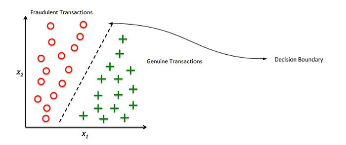
Logistic Regression Made Simple

Logistic Regression is a classification problem that finds out the probability of occurrence of data in either sides of a straight line or decision boundary.

It classifies the data points by fitting a straight line into the data

For drawing a line, Y=mX+c but we are not looking for Y, because we need a term that is going to give the probability on either sides. For that reason there is a concept of Sigmoid Function which takes any real valued number and map it into a value between 0 and 1. here’s the diagram of sigmoid function :

Sigmoid function or you can call logistic function will take X as an input and returns the probability. Why sigmoid? Its derivative is easy to calculate as it has a smooth curve.

This is the equation of a sigmoid function where e is the euler number , sigmoid takes X as an input and return the value between 0 and 1

We need to correlate the sigmoid function with the straight line because we are looking for the probability and not Y value. For that we substitute the equation of a line into the sigmoid function (logistic function).

We substitute the equation of a straight line ie mx+c into x and derive the equation

We get these results :

log(p/1-p)= mx+c , yes thats it. The equation of logistic regression.

We can correlate the straight line to the probability of occurrence by using a sigmoid function. By drawing a straight line to divide the data points and find the probability of occurrence on either sides (as in fig1). Hence we establish a relation between a line and logit function(ie log(p/1-p)) .

Cost Function

Based on the cost function/loss function , the model will try to learn and tune the hyperparameters for better predictions.

Cost function of Logistic Regression is called log-loss function/cross entropy

this hθ(x) is nothing but your predicted y ( predicted mx+c ) . You can also call it as y^ (hat) if it confuses you . y=> Expected y , m => Number of samples.

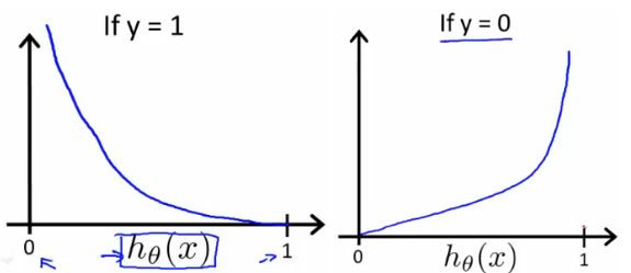
If it a binary classification, the cost function will be :

If we combine both these graphs, we get a graph like Gradient Descent Curve like below.

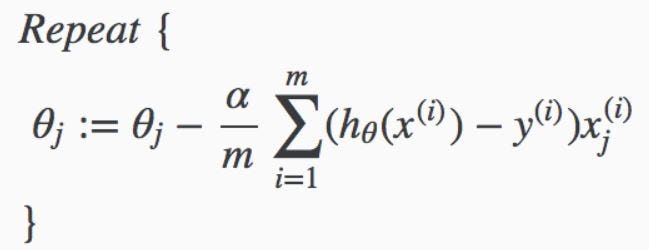
Wherever the concept of loss function comes, we somehow have to minimize the loss function that improves the performance of the model. Here to minimize the error we use the concept of Gradient Descent same as we used in Linear Regression.

After finding the cost function, we take the partial derivative of the cost function so the error will not change .

Partial derivative of cost function

We are taking the derivatives of cost function w.r.t ‘m’ and ‘c’ because , we want the points of ‘m’ and ‘c’ where the error will not change. For that we calculate the rate of change of error w.r.t to ‘m’ and ‘c’ and descent the points to reach the global minima .

Once we define these things we need to find the new value of m and c .

here Em and Ec is the partial derivate of cost function ie we calculate the derivate w.r.t m and c in the above equation.

Once we get the optimum value of m and c where the cost function is minimal or 0 we can draw best fit line in our logistic regression and convert those into the probabilistic function where values lies between 0 and 1 .

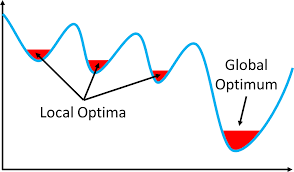
Note : We cannot use the cost function of regression because we will be getting a curve like this where there are many local minima’s.

This is a non — convex loss function.

Some tuning parameters of Logistic Regression are mentioned below.

click this for sklearn documentations.

penalty : default=’l2’ , Its an important hyper-parameter that helps you do the regularization .

C : default=1.0 , Large values of C give more freedom to the model. Conversely, smaller values of C constrain the model more. It controls the penalty of l1,l2 or elastic .

class_weight : default=None , We can add some weightage based on the target class if there is imbalance dataset , it should be passed in the form of dictionary .

n_jobs : Number of cores that is need to train the model.

Thank you all, hope you enjoyed the simple explanation!