What is Regression?
We first need to know what regression is ? What is a regression problem statement?
Regression is an important machine learning model technique for investigates the relationship between a dependent (target) and independent variable(predictor) where target variable will be continuous.
For example,

Here we predict the Weight w.r.t Age and Height , As you can see here our target variable (Weight) is continuous. Hence this is a Regression problem statement.
Now that we know what regression in Linear Regression is, lets start our topic,
Linear Regression Algorithm
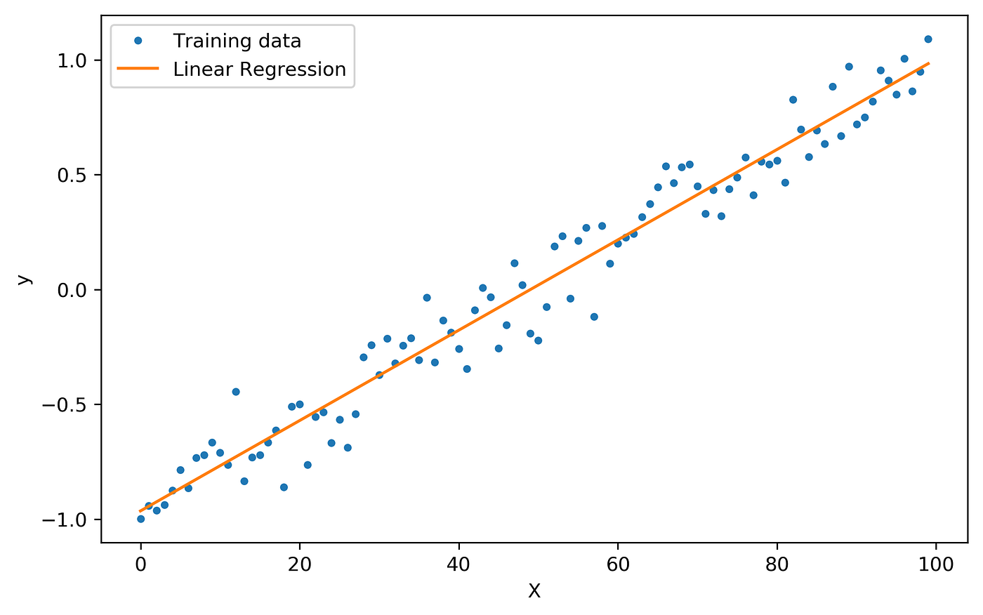
A Linear Regression Model predicts the dependent variable using a regression line or straight line based on the independent variables.
Easy, right?
We all know the equation of a straight line, Y= mx+c
where, m= slope/coefficient
c= intercept of the dependent variable
Y= dependent variable
With the help of a straight line we can draw the best-fit line for our dataset if our dataset follows a linear trend when we do the analysis(Exploratory Data Analysis).
Lets take an example and make it simple!!

We can say that , Height is directly proportional to Weight.

We can rewrite the equation in this way where e is the error rate .

We take two values and derive the value of m and c so that if we want to predict the new height we can do so by substituting the value of slope in the equation.
As i wanted to find the error, I substituted 5.3 and got the result 64. The expected result is 54 and we got 64. Here the error is 10(expected-predicted) Here we received this error because of m&c.
So we need to find the optimum value of m and c where the error is minimal, here is where the gradient descent comes into picture.Gradient Descent
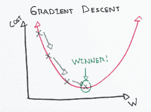
We have to shift or adjust the points in such a way that it touches the surface where the error is 0 /minimal (WINNER!!)
So that we get the new value/coordinates of m&c where the error is minimal for fitting the best fit line.
We cannot decrease the slope immediately because it will overshoot,we decrease it slowly at a particular rate.
Now getting back to the error/residual we got,
We got the error because our model couldn’t fit our data. We need to minimize the residual or cost function so as to get better prediction results.

Residual is a factor that pushes your linear model to find the value of m& c
Have a doubt on why we take the square and why not summation or modx?
- Because by squaring we ensures that each term is positive.
- If you take modx graph is given below, it is not differentiable at x=0.
- You can’t get derivative of modulus function because mod |x| graph is a Perfect V shape and in the graph we see a sharp point at origin.
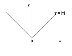
To differentiate, a function should have a smooth curve.
By squaring the term we get a smooth curve like as gradient descent curve(you can check the graph of x²)
So, the residual will keep on changing , so we take the partial derivatives of the residuals with respect to m&c.
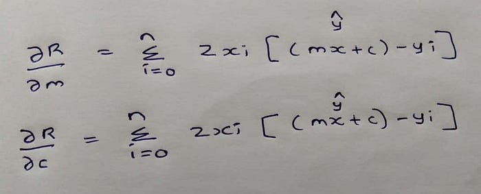
- We are taking the derivatives of the residuals with respect to m and c because we are finding the points of m and c where the error will not change.
- Gradient Descent will find the rate of change of residual w.r.t m&c and descent the points to reach the minimal point where error is low.
- Once we define these things, we need to find the new values of m&c and we will stop the process where dR/dm and dR/dc = 0 / minimal.
To find the new value of m&c,
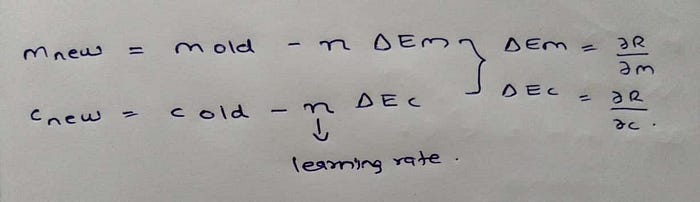
This will give you the new values of m and c . The learning rate is a tuning parameter in an algorithm that determines the step size at each iteration while moving toward a minimum of a loss function.
Once we get the new values of m and c where the error is close to 0 or 0 , we can draw a straight line where the error/RSS is minimum.
According to Google Tensor Board, Learning rate is between 0.00001 to 10.
- Higher Learning Rate will change the value of m and c by huge amount , it will be a problem for new data.
- Lower Learning Rate may never converge or may get stuck on a suboptimal solution.
Summary!
- We cannot decrease the slope immediately because it will overshoot,we decrease it slowly at a particular rate.
- Initialize the value of m and c ; Y=mx+c
- Find the residual/ error .
- Find the best value of m and c where the error will not change by taking the partial derivatives.
- Find the new values of m and c with the equation mentioned above.
- Once we get the new values of m and c where the error is close to 0 or 0 , we can draw a straight line where the error is minimum or repeat the process until we get the error as low.